Finding the celestial pole and aligning your telescope mount to it is something that any equatorial mount user knows well. There are different ways to go about it: visually through a polar scope (or with a dedicated polar scope camera), by measuring drift far away from the pole, or by platesolving near the pole. This last method - implemented in recent versions of SharpCap - is a quick and precise procedure and it is my favourite way to "polar align".
In this post I will explore the principles underpinning this approach. I make no claim to having invented this; my interest started with using SharpCap in which such polar alignment is implemented. Dr. Robin Glover (the author of SharpCap) credits the method to Dr. Themos Tsikas (@themostsikas) and his PhotoPolarAlign tool, which can be found on GitHub. What follows is my understanding of the method from reading PhotoPolarAlign source code, my user experience with SharpCap, and experimenting in Python. These notes will hopefully be useful to others interested in the topic.
My Python code, as well as images from a polar alignment session I did for testing, are both available on GitHub. The platesolving part was done with ASTAP, coordinate transformations with AstroPy, and numerical math with NumPy and SciPy. It's all relatively basic as far as astronomy/math goes, and it should be easy to implement given some astronomy library and platesolving software.
The Algorithm (From User's Perspective)
- Align the mount roughly to celestial pole.
- Take image A with the telescope in the upright position (RA=0°).
- Rotate the RA axis by about 90 degrees.
- Take image B with the telescope in the sideways position (RA=90°).
- Now the software knows where the RA axis is pointing on the celestial sphere. Iteratively apply corrections to the ALT/AZ base of your mount as suggested by the software, until the RA axis points close enough to the celestial pole. At every step, new image I is taken and suggested corrections are updated accordingly.
It is important to only change RA and ALT/AZ when prompted and never touch anything else (change DEC, rotate the camera, etc.). As long as the instructions are followed, you can get good polar alignment with a guidescope and guide camera.
The Algorithm (From Software's Perspective)
- Platesolve image A (that is, find transformation from "local" pixel coordinates to "world" RA/DEC coordinates), setting its center as point $A$.
- Platesolve image B, setting its center as point $B$.
- Find the origin ($R_0$) of a rotation that transforms coordinate system of image A to that of image B (that is, find a point that has the same "world" RA/DEC coordinates and "local" pixel coordinates in both images).
- Find the celestial pole coordinates ($CP$).
- Compute relative position of $R_0$ with respect to $CP$. This is the initial error / suggested correction.
- For "improvement" image I1 and subsequent images Ii:
- Platesolve image Ii, setting its center as $I_i$.
- Find the relative position of $I_i$ and $B$ and apply this offset to $R_0$, creating new point $R_i$.
- Compute relative position of $R_i$ with respect to $CP$. This is the improved error / suggested correction.
(In the following text I will discuss two implementation variants of this general idea: the "simple" version and the "improved" version.)
Step 3 is where the "magic" happens; once we know the initial position of the RA axis, we can compute what offset is necessary and guide the user through the ALT/AZ changes.

Some Caveats Of A Naive Implementation
Looking at it in more detail, there are some considerations:
- For "world" coordinates given as RA/DEC, there is a difference between the reference equinox (J2000) and observation time. The North celestial pole is not at RA=0°, DEC=90° in the J2000 reference frame (as of 2021, anyway). Platesolving will probably give you J2000 coordinates. This is what Step 4 refers to.
- The Earth moves! Platesolving computes RA/DEC coordinates, but we're trying to correct ALT/AZ. Unless the whole procedure is instantaneous, there will be some drift in the images which you may want to compensate for. (The movement in RA axis is about 360° per 24 hours = 15° per hour = 15 arcmin per minute, however this only translates 1:1 to "great circle" distance at the celestial equator, the distances near the pole are much less).
- The total alignment error can be computed equally well in any spherical coordinate system (eg. RA/DEC J2000), but the per-axis corrections are best given in ALT/AZ. This can be achieved using proper RA/DEC to ALT/AZ conversion (using observation location and time), or by using the local coordinate system from image A (according to the instructions, the horizontal axis should be roughly azimuth, the vertical axis should be roughly altitude).
- Transforming "local" pixel coordinates to "world" RA/DEC or ALT/AZ coordinates involves projecting a plane onto a sphere. With the Gnomic projection this means that image scale is actually not a constant, but increases with distance from the center (imagine an ultrawide rectilinear lens). Measuring angular distance in pixels, particularly with points far outside of the image FoV, will incur an error compared to the true "great circle" distance. (This may still be negligible, as in of the order of a single pixel for relevant image scales and distances, though).
- Atmospheric refraction means that the true celestial pole is in a slightly different location than it appears to be. This effect is altitude dependent (objects lower in the sky are more refracted; observation sites closer to Earth's equator will see the celestial pole lower in their sky and thus more affected by refraction).
The Core Idea - Solving The Rotation
Beauty of the PhotoPolarAlign method is in that it doesn't require you to:
- know the exact initial RA/DEC (mis)alignment of your camera, or have it be fixed to the RA axis,
- know the exact amount rotation in RA you perform,
- see the celestial pole (or any particular stars) in your image.
All you need is two images in different RA positions, and the algorithm figures out the axis of the rotation from that, even if it is outside the view.
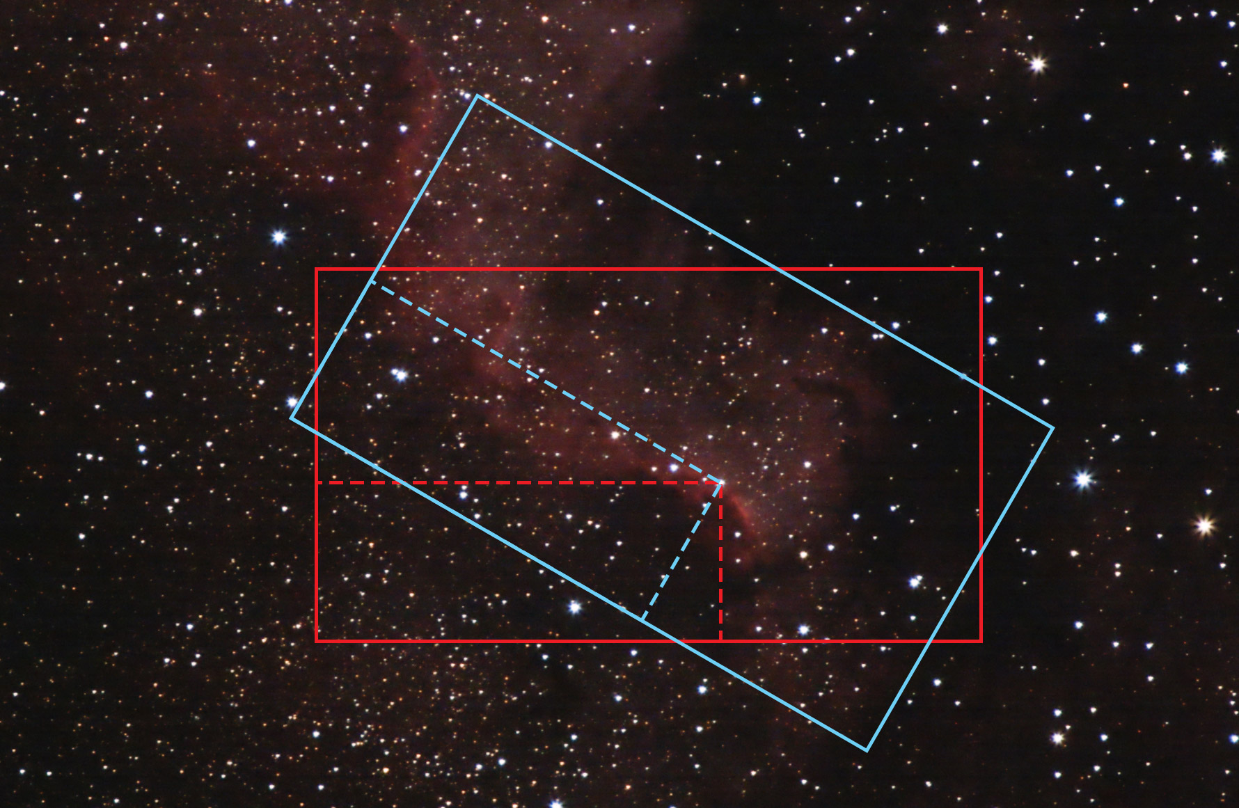
For simplicity, let's look at the case when the center of rotation is visible first. It must be visible in both images, because it's the only point which doesn't actually move with the rotation. Points around it experience a little movement, more distant parts of the image have even more movement (as measured by difference in "local" pixel coordinates for a given fixed "world" coordinate, eg. a star). The amount of movement is proportional to the rotation angle, but any non-zero angle gives the same general structure: a single point with no movement, and movement increasing with distance from that point.
Let's consider the more general case when the center of rotation is outside the field of view. Platesolving in ASTAP gives the Gnomic (rectilinear) projection, so that we know where the view is pointed on the celestial sphere and what is its rotation. The projection is valid regardless of focal length or sensor size - these just determine what "central crop" of the projection plane is visible (in a world with perfect optics, etc.). The center of rotation may lie on local coordinates which are outside the image/sensor, but if we just had a larger sensor, we would see it at those coordinates.
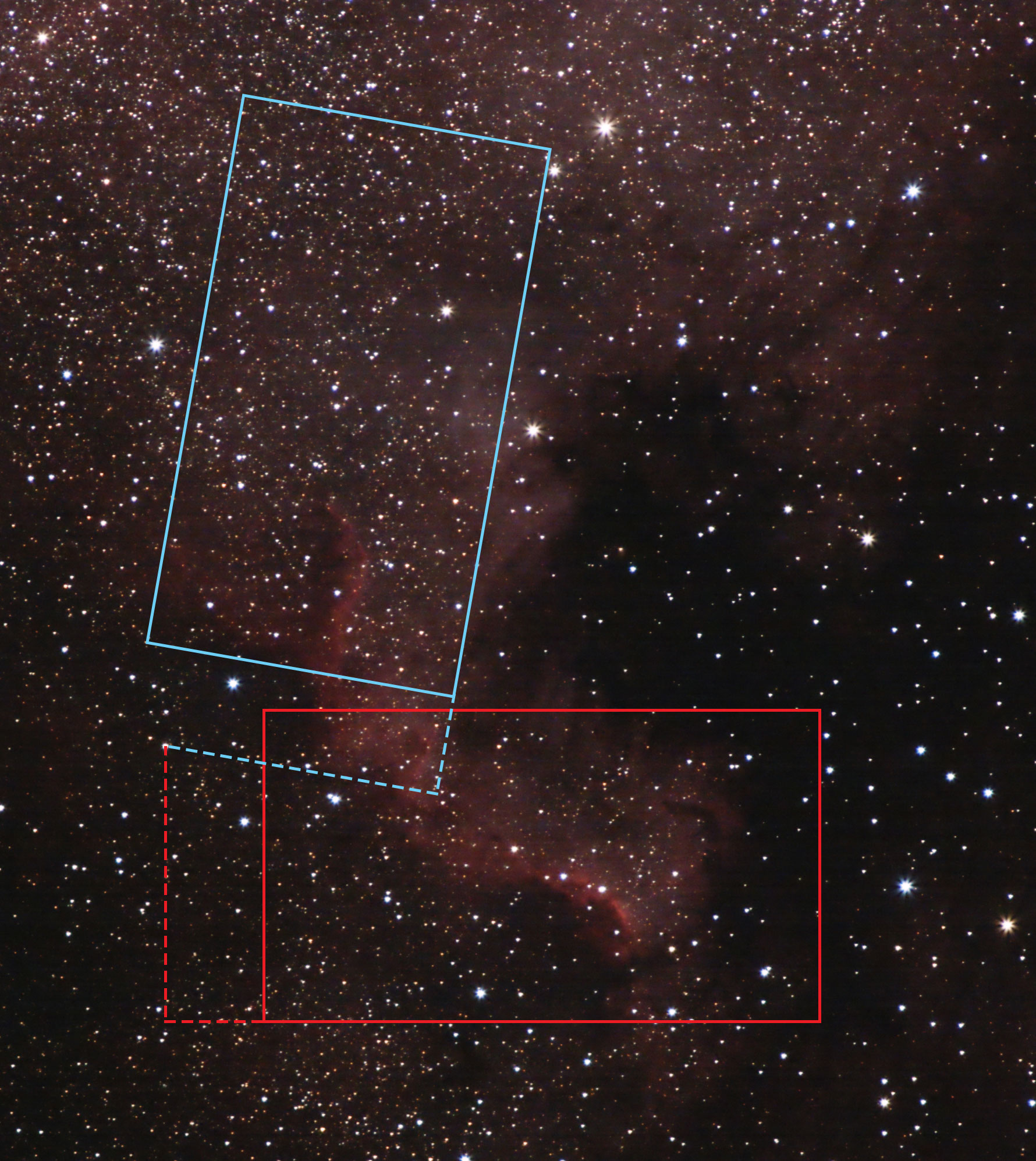
Practically speaking, we need to find a fixed point of the rotation, which is the point (in global coordinates, let's say) that minimizes distance between its images in the local coordinates. There should be a single global minimum with distance zero.
This optimization problem can be solved numerically. It can be practical to formulate it in terms of image A local coordinates. It looks pretty well-behaved.
The original PhotoPolarAlign implementation (link to relevant part of code) uses Broyden's method to solve it, though I guess any reasonable algorithm will be able to handle it; there is little need to get very precise solution, as the differences will be orders of magnitude smaller than one pixel.
The original implementation finds the root of function $f(x_A, y_A) = (x_A - x_B, y_A - y_B)$, where $x_A$ is a pixel coordinate in A and $x_B = x_B(J2000(x_A, y_A))$ is the same "world" point represented as pixel coordinate in B. I've tried to do the same with minimizing squares: $f(x_A, y_A) = (x_A - x_B)^2 + (y_A - y_B)^2$ and Nelder-Mead and got effectively the same solution.

The graph above shows the problem space for the sum of squares formulation. The distance between $R_0$ coordinates in A and B is $\sqrt{3.3\times10^{-9}}$ pixels, ie. about 0.0001 arcseconds.
Analyzing A Polar Alignment Session
To better understand the method, I've recorded a polar alignment session in SharpCap with a 280mm guidescope mounted on iOptron SkyGuider Pro (which itself was turned off), giving just over 1° FoV as recommended by SharpCap. Data is available here on GitHub.
I'm aware of two caveats regarding the data:
- The location entered in SharpCap settings was a bit off (in SharpCap: 50.2N, 14.9E; in reality: 50.1N, 14.4E). I'm not sure how much difference does it make. I did not use the refraction functionality.
- I didn't test the resulting polar alignment with other method to try and quantify the error. In my experience, SharpCap alignment works pretty well, but due to the indirect nature of the method it's not obvious from the data that the results are correct.
| Observation site | approx. 50.1° North, 14.4° East (Prague, Czech Republic) |
|---|---|
| Observation time | around 2021-05-31 00:30 GMT+2 (2021-05-30 22:30 GMT), 15 minute session |
| Telescope | ZWO 60/280 finderscope (link) |
| Camera | ZWO ASI 290MM mini (link), 1936 × 1096 pixels @ 2.9 μm |
| Mount | iOptron SkyGuider Pro (turned off) w/ iOptron AltAz base, on photo tripod |
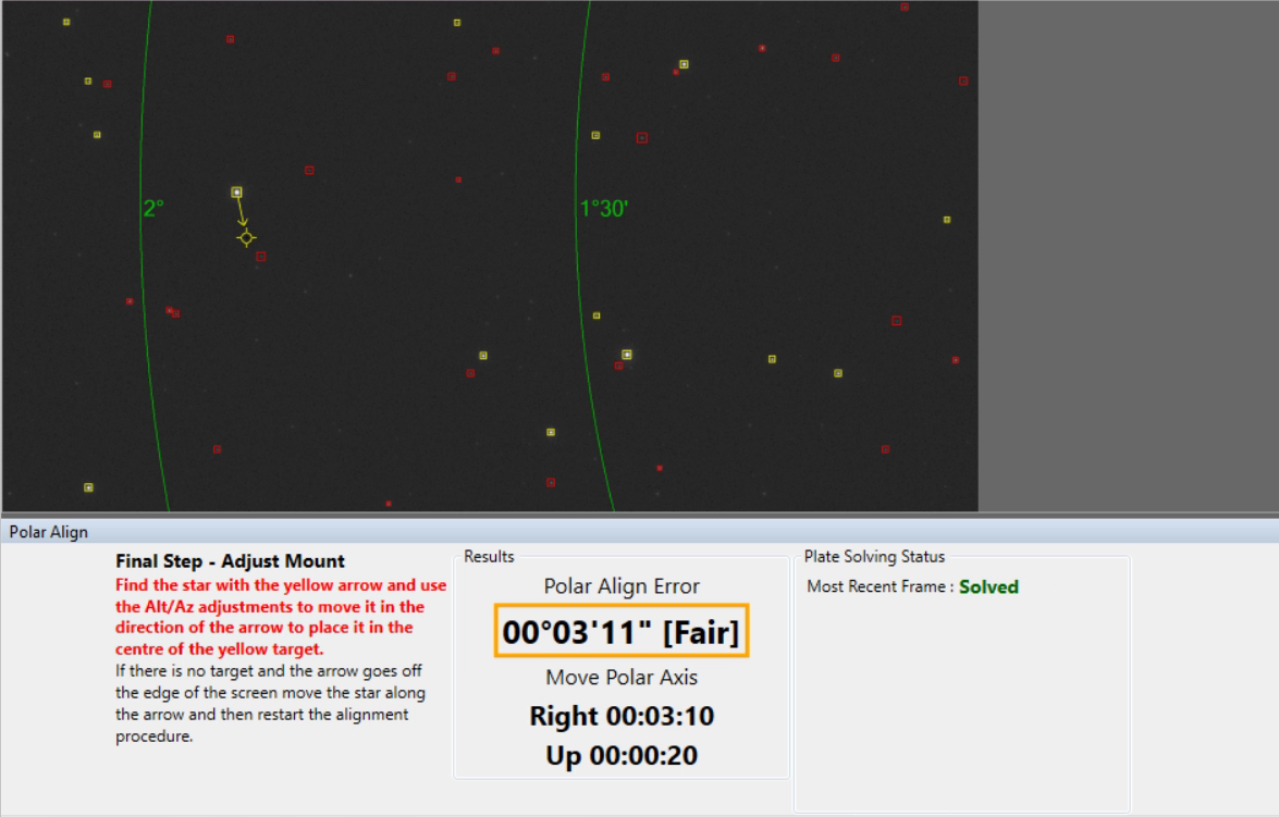
According to SharpCap, the inital alignment error was 3°50'44", with the final error being about 20" or Excellent, as described by SharpCap. (It's always nice to see the dark green box after fiddling with the iOptron base.) Though the math works out to precise numbers, it feels most natural to me to measure the error in arcminutes. This is the session as evaluated by SharpCap:

Note that the adjustments have been guided by these SharpCap results, with the goal to minimize error as reported by SharpCap.
The "Simple" Implementation
I implemented the algorithm described above using Python, AstroPy and ASTAP. In this "simple" version, I'm:
- using RA/DEC J2000 coordinates as they come from the platesolving, without considering rotation of the Earth between frames (note the whole session lasts 15 minutes), and
- working in "local" coordinate space of image A (pixels), measuring angular distances with pixels and assuming that X/Y are aligned with AZ/ALT.
When evaluating the pictures I recorded during the live session with SharpCap, I got this result:

The evaluated error gets down to about 6'45" before settling at 13'30"; a major difference to SharpCap's result of 20". Comparing the data you can see a large offset in AZ as well as the error increasing over time compared to no such trend in the SharpCap dataset.
The "Improved" Implementation
After more experimentation I arrived at what I call the "improved" version. This one more closely follows PhotoPolarAlign code and adds one additional refinement not present in PhotoPolarAlign.
In the "improved" version:
- after finding $R_0$, everything is done in ALT/AZ coordinates, using actual observation time of each image (Earth's rotation is accounted for, no error due to projection distorsion in measuring distances), and
- in the $R_0$ finding procedure, Earth's rotation is also accounted for when projecting from pixels in A to RA/DEC and back to pixels in B.
The second point is not done in PhotoPolarAlign. I've implemented it so that it can use the existing RA/DEC J2000 projection to/from pixels, so it's not actual ALT/AZ, but the movement should be virtually the same. In the test session (which has 1 minute delay between A and B images) it has a minor effect on the error compared to SharpCap.

The evaluated error gets down to 30" before settling at 1'25". This is the closest I was able to get to the SharpCap results, and after the initial disappointing numbers it looks like a viable implementation. Note that these are results from one session, using one image scale, without independent verification of the error. However, it looks to me that it behaves quite similarly.
Without compensating Earth's rotation in computing $R_0$ it looks like this:

The results are a tad worse, both in terms of the total error (gets to 1"12', final 1"38') and looking at the AZ/ALT axes. The $R_0$ correction seems preferable.
Appendix: The "Simple" Implementation In Python
Below is the main code of my "simple" implementation, you can find the full code on GitHub, including the "improved" variant.
See also the original PhotoPolarAlign on GitHub, which includes its version of the algorithm as well as GUI.
# All values "*_pix" are given in A local coordinates (ie. pixels)

# step (1)
A_J2000 = get_J2000(A)
A_pix = J2000_to_pix(A, A_J2000)

# step (2)
B_J2000 = get_J2000(B)
B_pix = J2000_to_pix(A, B_J2000)

# step (3)
def displacement_error_squared(pix):
    coord = pix_to_J2000(A, pix)
    pix2 = J2000_to_pix(B, coord)
    return np.sum((pix - pix2) ** 2)

res = scipy.optimize.minimize(displacement_error_squared, A_pix, method="nelder-mead")
R0_pix = res.x
R0_J2000 = pix_to_J2000(A, R0_pix)

# step (4)
NCP_J2000 = SkyCoord(ra=0, dec=90, frame='fk5', unit="deg", equinox="J2000")
NCP_to_date_J2000 = SkyCoord(ra=0, dec=90, frame='fk5', unit="deg", equinox=get_time(A)).transform_to(FK5(equinox="J2000"))
NCP_to_date_pix = J2000_to_pix(A, NCP_to_date_J2000)

# steps (5), (6)
for I in all_image_names[1:]:
    I_J2000 = get_J2000(I)
    I_pix = J2000_to_pix(A, I_J2000)

    offset_pix = I_pix - B_pix
    Ri_pix = R0_pix + offset_pix
    Ri_J2000 = pix_to_J2000(A, Ri_pix)
    error_pix = Ri_pix - NCP_to_date_pix
    error_arcmin = error_pix * arcsec_per_pix / 60